A Clockwork Egg

Every morning, I cook scrambled eggs. After years of repetition, each step in my routine is automatic. If I turn on the burner before I walk to the fridge, the butter will be just starting to bubble when I finish beating the eggs, and I can clean the mixing bowl in the brief pause before they're ready to be stirred. Anyone with a morning commute can relate to this mindless optimization—if you do the same task a thousand times, you stumble on tiny improvements through the trial and error of random variation. Once formed, these habits are unlikely to change, until there's an external shock.

Forced Experimentation

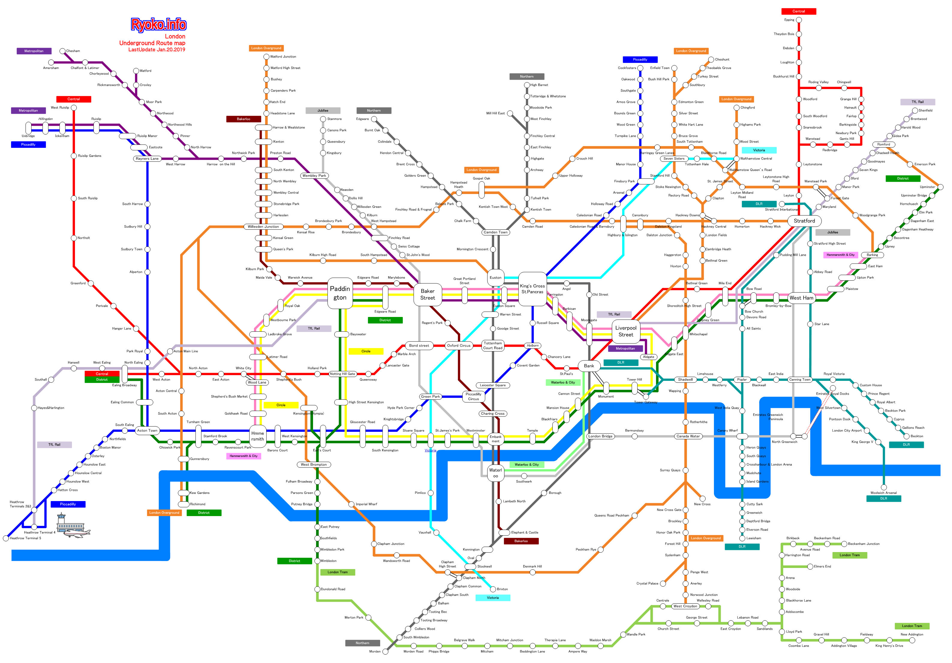
On February 4th, 2014, the London Tube workers went on strike, forcing a number of station closures throughout the city. For three days, some commuters were unable to take their usual route to work, and were forced to find alternatives. After the strike, the stations reopened, and life could go back to normal.

Three economists saw the opportunity for a natural experiment—only certain commuters were disrupted by the closure, and using the subway's tracking data, their movements could be compared to the unaffected group. Surprisingly, life didn't go back to normal after the strike ended. Instead, some of the disrupted group realized they had stumbled onto a faster route during the strike, and they didn't switch back. In fact, researchers even claimed that the time savings from these discoveries were so significant that the strike caused a net decrease in time spent commuting, despite the initial disruptions.¹ Even if only a small fraction found new routes, the benefits from their new routine would accrue over years to come, while the initial disruption was brief.

This post will explore how this story can be naturally understood through the lens of mathematical optimization. In fact, there are deep parallels between this theoretical framework and the problems we confront in our daily lives. This proves useful in both directions—the intuition we have built from lived experience helps us learn the mathematical theory, while that mathematical theory can in turn identify the limitations of our intuition.

We will use a trio of real world examples—this subway strike, the quest for the perfect cookie, and the search for the top of a mountain—to illustrate the basic building blocks of optimization. Then, we'll explore the surprisingly rich implications of random noise (like, perhaps, a subway strike) within optimization algorithms.

The Framework of "Optimization"

Math always starts with a definition. The DeepAI website writes the following.

Mathematical optimization is the process of maximizing or minimizing an objective function by finding the best available values across a set of inputs.

It's easiest to explain these terms by example.

• For London commuters, their "objective function" might be the duration of the commute,² and the "available values across a set of inputs" might be the route they take.
• If we want to find the highest peak in a mountain range (an example we'll discuss in detail in the next section), the input would the latitude and longitude of a point on the map, and the objective function would be the elevation at that point.
• When baking chocolate chip cookies, the possible inputs might be the amount of each ingredient and the order in which they are combined, and the objective function might be the tastiness of the resulting cookie. This isn't a joke—Google once ran a cookie optimization experiment along these lines.³

Optimization is one of the most common tasks in applied mathematics, but finding solutions can be hard. The vast increase in computational power has broadened our horizons for what optimization challenges are feasible, but many important problems remain out of our reach.

In an optimization problem, we typically assume that we are able to check the value of the objective function at some chosen input (often called "queries" to the objective function, or perhaps, the "oracle"). For example:

• We can follow a certain route on the subway and use our stopwatch to record the duration of the trip.
• We can bake a batch of cookies following a certain recipe, and taste them.
• We use ElevationBot 1.0, a simple computer which takes in a pair of latitude and longitude coordinates, and spits out the altitude of that point.

A naive optimization strategy is to simply try a bunch of inputs, and hope that we find a good output. For instance, we define a grid of latitude and longitude coordinates, feed these coordinates into ElevationBot 1.0, and use the that highest point we find as out answer. But this naive approach only works when the range of potential inputs is sufficiently narrow. In particular, we need to consider the "dimension" of the input space. The number of points within an exhaustive "grid" of inputs grows exponentially with the dimension of the input. Latitude and longitude represent a mere 2 dimensions, so the number of points in our grid is just the square of the number of points per side. However, the famous Jacques Torres cookie recipe has 12 ingredients. If we wanted to try all combinations at a mere five different amounts of each ingredient, that require over two hundred thousand possibilities (which is a bit much for even a hungry baker).

In our own lives, we often confront similar optimization challenges, but we rarely take this naive approach. Instead, we typically to look around us for small local optimizations, whose benefits we can easily identify.

Locality in Optimization

Imagine biting into a warm cookie, fresh out of the oven. The rich buttery center has just the right chew, while the edges are lightly crisp. You taste the faintest hints of toffee, butterscotch, and vanilla, and the sprinkle of sea salt on top adds an extra kick. It's almost perfect, but there's not quite enough bite from the dark chocolate.

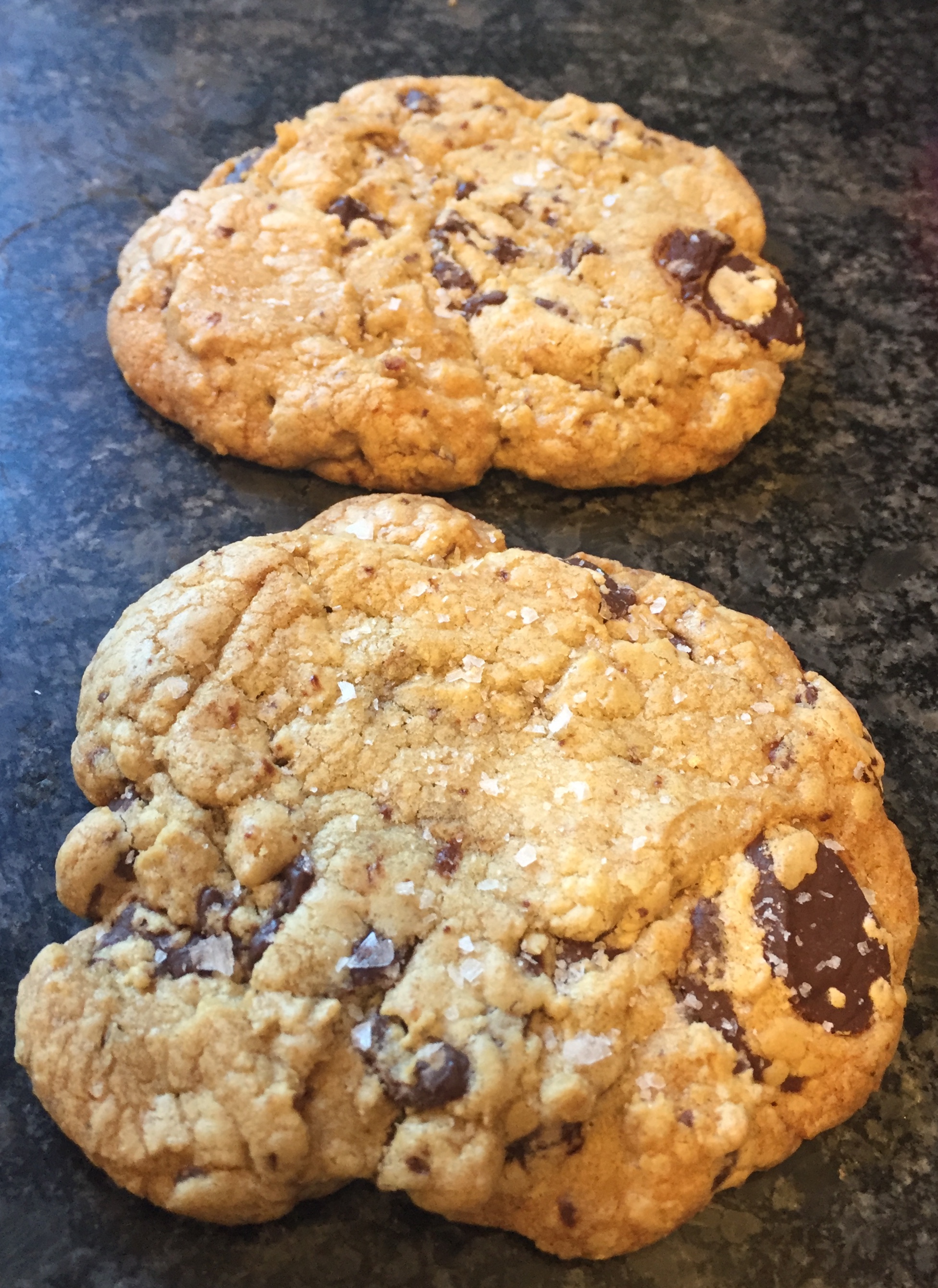
We wouldn't just throw up our hands and start from scratch… we'd just add more chocolate! The average baker can't look at a cookie recipe, and imagine exactly what the result will taste like from afar. But we can taste a recipe, and imagine what a small specific tweak would do to the result.

"Locality" in optimization refers to "closeness" in the input space. In latitude and longitude, this would be the "as the crow flies" distance, while in the input space of "cookie ingredients" and "subway commuting choices", the definition is a bit less rigorous, but we can still imagine what constitutes a "small" change. In general, we can estimate the impacts of a single small single change to the input, but not multiple big adjustments. If we increase the amount of chocolate, we know they'll taste roughly the same as before, but a bit more chocolate-y. If we increase the amounts of chocolate, butter, and baking soda, cut some flour, and tweak the balance between brown and cane sugar, can the typical home cook really guess what the result will taste like?

In the London Tube experiment, the researchers lay some of the blame on the "stylized nature" of the Tube map displayed to commuters. Its spatial distortions make it difficult to spot major inefficiencies in their route, without some external push. By comparison, we can usually estimate the impact of these "local" changes by ourselves. If we get off one stop earlier, maybe our walk to work increases by a minute, but we avoid the wait at a crowded station. These slight changes are a bit like tweaking just a single ingredient in a cookie, and we might be able to tell whether or not they are worth trying.

Before, we imagined a challenge where we tried to find a peak of a mountain range, using ElevationBot 1.0, which could tell us the elevation of any point defined by its latitude and longitude. Now, let's imagine that there was an upgrade to ElevationBot 2.0, which also tells us the slope of the incline of this point (that is, "which direction slopes downward, and how steep is it", often referred to as the gradient). This better reflects our intuition for local optimization in other settings, but it's also not a terribly difficult task for the ElevationBot, as the diligent machine could always query the elevation at nearby points, and use those to form an estimate of the local slope.

Now, imagine that we were hiking with an altimeter, and we can look around and see the direction of the hillside slope around us. However, our information is strictly "local"—we're stuck in the foggy forests of the Appalachians, not the wide open granite of the Sierra Nevada, so we can't look miles away to spy what peak might be highest. How might we find the highest peak? Well, our intuition is simple: from wherever we are, we choose to "go up". This "algorithm" is called "gradient ascent".

Gradient Ascent

Gradient ascent is a canonical optimization algorithm, and the step-py-step process can be described as follows (its simplest summary is simply "go up, as fast as you can"):

• We begin at some initial point.
• We find the direction of steepest ascent from that point, i.e. "if you took a few steps in any direction, which would make you gain the most elevation?" (the magnitude and direction of steepest ascent form the "gradient", and the direction is the opposite of where a marble would roll).
• Then, we walk for some distance in that direction (this amount is referred to as the "step size", meaning a step of the algorithm, not a step with your feet).
• Once we finish walking, we look around our new location, and we repeat this process again (i.e. determine the direction of steepest ascent, and walk in that direction).
• Once we reach a point that is essentially flat, there is no direction we can follow which takes us any higher, and we are done (this is called "convergence").

To see this written in basic mathematical notation, see Appendix: Gradient Ascent Algorithm.

This isn't some arbitrary example—it's a natural definition of what it means to improve our situation through local changes. Wherever we are, we ask "what small change could we take to make to make this better?". If these cookies were too salty, then next time we would simply use a bit less salt, rather than starting completely fresh from a new recipe.

Visualizing Gradient Ascent

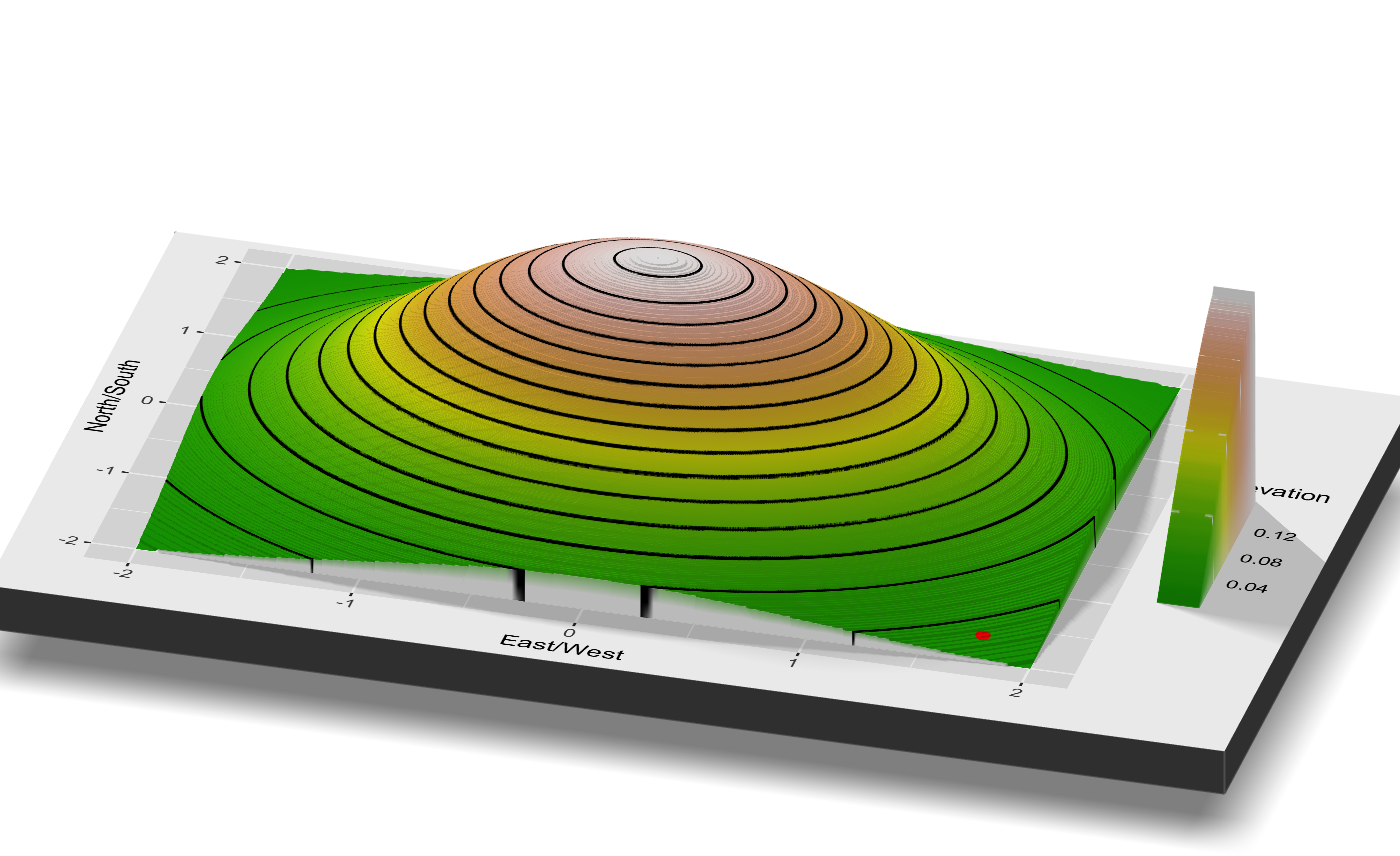
So, we follow the direction of steepest ascent, but what does that look like in practice? We can visualize our challenge of finding the highest point in a very simple mountain range. In fact, simplest of all, imagine a single hill. This one is perfectly round, but we pretend we don't know that, and we can only see the local area around us.

The following is a contour plot, like what you find on a topographical map. At the center is the highest point, and it slopes down as you get further away. Our current position is the red dot, in the southeast.

It might be more clear if we consider viewing the map at an angle (thanks to the rayshader package.

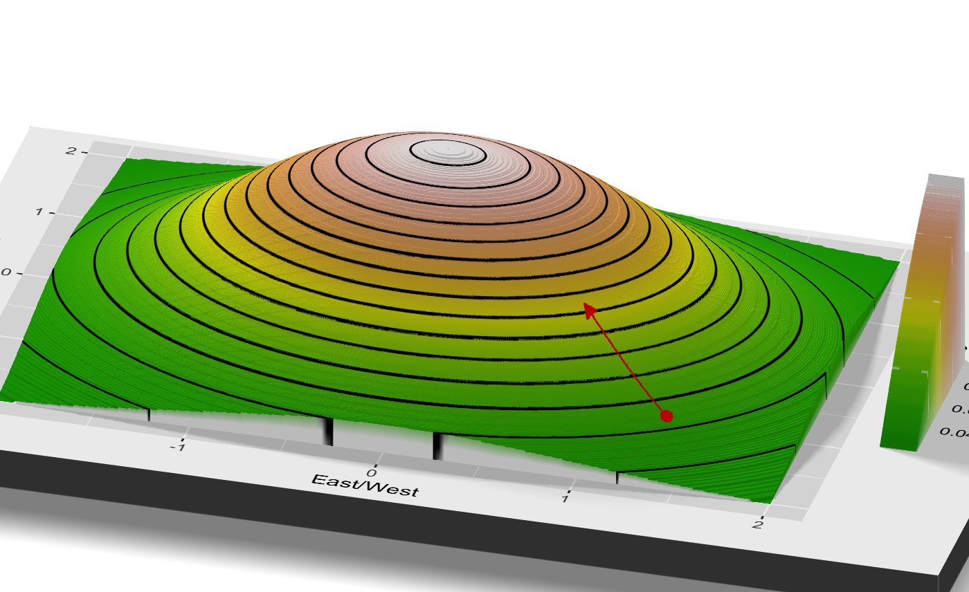
Let's imagine gradient ascent in action. We look around, and see that the direction of steepest ascent is to the northwest, shown by the red arrow.

We move that distance up the slope, and look around once again. We see that the direction of steepest ascent is still northwest, so we move once more.

Or, shown in 3D (which is admittedly hard to draw…).

We repeat this process until we look around for that direction of steepest ascent, and see that we're at a point which is basically flat. You can watch the whole process in the gif below. We start in the bottom right, and climb and climb until we reach the top of the mountain, where we stop.⁴

Not All Mountains Are Friendly

In this simple example, our local minimization strategy ("just go up!") finds the highest peak without any trouble. However, imagine there were three different peaks, of differing heights.

It's a bit harder to picture, but a 3D visualization might help show the shape.

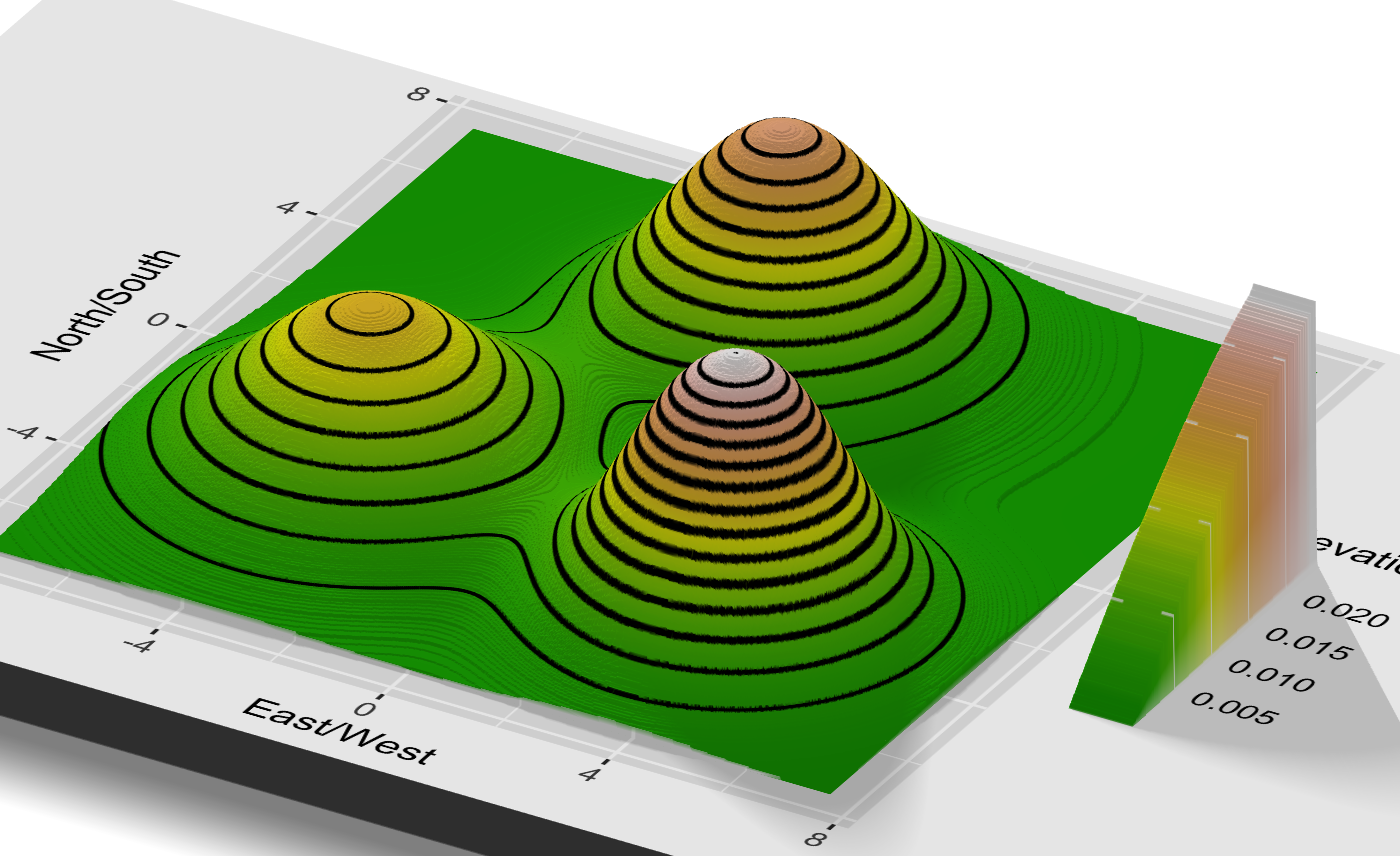
This poses an obvious problem for our algorithm. We hike up until we reach the top of a peak, look around, see that we can't go up any further, and stop. But this could be true of any of the three peaks, and only the peak in the southeast is actually highest.

Let's say we start near the center of this region, and follow our algorithm. We climb up south and to the east, and reach that highest peak, just like as we did in the case of a single hill.

However, what if our starting position was just a bit further north? Well, in the gif below, we see that we'd head off in the opposite direction, and end up at the northmost peak. We'd halt at the top, unable to climb any further, and be forever stuck at a lower point than the peak in the southeast. And by the rules of our game, we can only see the area around us, and we'll never know that there's a higher peak elsewhere! And most crucially, we couldn't possibly tell the difference between the two starting points, without prior knowledge of the area.

This illustrates a fundamental divide in mathematical optimization. Some surfaces are "convex", which ensures that gradient ascent will march us directly to the highest point (the "global maxima"), no matter where we begin.⁵ However, "nonconvex" surfaces lack such guarantees, and might prove computationally intractable (any "mountain range", by definition, falls into this category, as it has multiple peaks). Informal definitions of these terms can be found in the appendix (Appendix: The Perils of "Nonconvexity"), but the most intuitive takeaway is the issue of "spurious optima". To clarify the jargon…

• Optima: either maxima or minima (these challenges are equivalent).
• Global optimum (or maximum/minimum): the optimum among the entire input space
• Local optima (or maxima/minima): these points are optima in a small neighborhood around themselves, but not if you consider points far away. There is no local direction which takes you higher (or lower, if minimizing), but none are the global optimum.
• In the context of optimization, local optima are also called spurious optima, because they have the same local properties as the global optimum, but they are not the solution to the optimization challenge.

In the convex realm, local information provides us with global guidance, and we can follow the path of steepest ascent all the way to the maxima. In the nonconvex setting, we might instead find ourselves trapped in a spurious optima.

Not Settling for Second Best

If we are wary of getting stuck at a spurious optima, how can we modify our approach to ensure we find the highest peak?

Well, we saw above, that certain starting positions were successful, and others lead us astray. What if we simply used our gradient ascent algorithm multiple times, starting from randomly chosen starting points? Then we could check the results of each of our attempts, and pick the highest point we find. The gif below shows what that might look like.⁶ If we try a number of randomly chosen points, we are highly likely to find one that leads to the highest peak.

In a sense, the challenge becomes one of initialization. This is common in the optimization literature. Even if the optimization surface is nonconvex, we just need to find a starting point that's reasonably close to the optima (within its "basin of attraction"), and our naive gradient ascent algorithm can do the rest. Countless papers have been written on the topic.

It's also a natural fit for our intuition—if you set out to find the perfect chocolate chip cookie, I bet you'd do something similar. You might start with a few different recipes that look promising, and then try and find small improvements based on the results (a bit less salt, or a bit more chocolate). It's the equivalent of trying different starting points, and then following gradient ascent. In this case, it's intuitively clear why "random initialization" would be a poor choice—we know a great deal about what makes for a good chocolate chip cookie, and it'd be foolish for us to not leverage that (e.g. picking the ingredient ratios at random, rather than following proven recipes).

Thus, the challenge boils down to how hard it is to find the right starting point. Are any of the popular cookie recipes out there reasonably close to your own personal, optimal cookie? Hard to say. A large region of the mountain range above leads to the best peak, but what if there were dozens of mountains and the tallest one was steep with a narrow base? The difficulty of optimization always depends on the unique shape of the setting.

Embracing Random Noise

Or, we could view the challenge from a different perspective. Instead of trying to optimize different starting points using their local information, what if we were a bit more flexible in our climbing path and were willing to experiment along the way?

Of course, there's a reason that gradient ascent is so rigid in its path—it always goes in the direction that gives you the largest gain in the shortest amount of time. Any other direction appears inferior. If the cookies aren't chocolate-y enough, you'd feel a little silly trying any other fix besides adding more chocolate chips to the dough. But as we've seen, local improvements will only take you so far. My ideal chocolate chip cookie is thick and chewy, but imagine that I had only ever tried recipes which were thin and crispy. I could try and improve them by tinkering with the balance of butter and sugar, or adding more chocolate, which might make them taste a bit better. But, it would require the simultaneous change of many ingredients to make the huge leap from one type of cookie to the other.⁷

What if we were a little more open to experimentation, even if we can't easily see how it would help? Let's recall the example of the London subway. These commuters had settled into their preferred morning routes, and surely if they could spot any tiny tweak which would save them time, they would have already tried it. The three-day strike represented an external shock to the system, which pushed them out of their local equilibrium. It wasn't designed to improve their commute (if anything, it was the opposite). And yet, by random chance, a group of commuters found themselves pushed into a surprisingly superior path, which they stuck with. Only through this forced random experimentation did they escape their local optima.

What might this look like mathematically? Well, we could introduce random "noise" into our movement. Let's imagine gradient ascent once more. From our starting point, we walk in the direction of greatest ascent, and then, we walk a bit further in a random direction. This won't feel very rewarding in the moment… we want to go "up", we can see which direction takes us "up", and yet, we go in a random direction? But, maybe this extra experimentation will give us a chance to escape our deterministic march towards a spurious optima, and we will eventually find the highest peak. We will still tend to go "up", but we might not follow such a direct path.

To be mathematically precise (again, you can just skip the mathematical part if you'd like), we simply add the random noise to our gradient ascent step from before. That is, now we set \(x^{(k+1)} \leftarrow x^{(k)} + \eta \nabla f(x^{(k)}) + \sigma^2 \epsilon_k\), where \(\epsilon_k \sim N(0, 1)\). That is, we add a normally distributed random noise term to each gradient ascent step.

To visualize this, we turn to the one dimensional case. A one-dimensional mountain range might not be quite as intuitive, but it's a lot easier to see on your screen, and the same rules apply. Below, we consider a mountain range where the middle peak is the highest. Following gradient ascent, if we start on the far right, we quickly find the nearby peak, but are stuck there, unable to find the highest point.

However, if we start from the same place, but add a bit of noise with every step, our path isn't quite so direct. We take a bit longer to reach the top of the low peak, but from there, the random noise gives us a chance to "escape". That is, with each move, we feel a pull back towards the low peak (as that is the direction of ascent). But if we get lucky, and find a sequence of random noise terms that "push" us far enough to the the left, we escape this valley and feel the pull of the highest peak. The addition of random noise allows us to escape eternal mediocrity, stuck at the top of the low peak.

Of course, this gif takes a long time to run—it requires a very lucky sequence of steps for us to escape the local optima! Thus, this is far from an easy fix. In fact, this highlights the importance of precisely tuning this approach. Blindly adding random noise will eventually let you find the summit, but along the way you'll be stuck with long stretches of experimentation before you get anywhere.

Estimation Error as Noise

Simply adding random noise to gradient ascent isn't a "real" algorithm that would be ever used in practice, but it helps illustrate the powerful premise of "stochastic optimization" (i.e. optimization techniques which leverage random chance). Many varieties of stochastic optimization see widespread use,⁸ but here, I'll focus on one particularly relevant example: Stochastic Gradient Descent (SGD).

The premise of Stochastic Gradient Descent is a natural extension of the gradient ascent algorithm we studied above. First, we note again "gradient ascent" and "gradient descent" are equivalent—you simply take the negative of the gradient to switch between maximization and minimization. Rather, it's the "stochastic" that's new.⁹ In gradient ascent, we needed to compute the slope of the local area (i.e. the gradient) with each step. Let's consider again our ElevationBot 2.0 which takes in latitude and longitude coordinates, and tells us the elevation and local slope of that point. But perhaps we're not the only ones trying to play this addictive "find the highest peak" game, so we have to wait in a long line before each query. However, nearby we see a rusted old ElevationBot 1.5 terminal. It's an intermediate model, between version 1.0 (which just computes the altitude) and 2.0 (which also computes the direction of ascent), because it can only estimate the direction of ascent, and it's occasionally a bit off. However, there's no one in line to use it, so we can rattle off our queries much faster. Should we skip the line and use the faster but less reliable estimates of the 1.5 model?

This silly story might make the setting sound overly contrived, but it's actually a very foundational trade-off. It is often much faster to compute an approximate slope rather than an exact one.¹⁰ This is the premise of Stochastic Gradient Descent—the exact gradient is replaced by a stochastic gradient, which is much faster to compute but is only an approximation of the truth.

This is no niche use case. Stochastic Gradient Descent has been the industry standard technique for optimizing artificial neural nets for decades. When you hear about the rise of "deep learning" in the news, Stochastic Gradient Descent is the most reliable and versatile computational tool in the field. The challenge of neural networks is that their optimization space might consist of millions of dimensions (above, we visualized optimizing over a single dimension!). In fact, Microsoft recently boasted of a neural network with 17 billion (!) dimensions. The inevitable result of these optimization structures is that there are an enormous number of spurious local optima.

This begs the question: if neural networks are loaded with spurious local optima, and following the gradient will often lead to those spurious points, then in the words of neural nets pioneer Geoffrey Hinton, why does SGD work so "unreasonably well"?

There are a variety of answers, depending on whom you ask, but the most common reason researchers point to (an explanation dating back decades), is that the inherent noise in the imprecise stochastic approximation allows it to escape spurious local optima.¹¹ This is not noise that we added explicitly—it's just the approximation error that arises from not computing the exact gradient. And yet, these random shocks turn out to be an advantage, rather than a hindrance. Even at the computational cutting edge of the field, random noise can be a powerfully helpful force, pushing us away from spurious optima and towards our goal.

Wrapping Up

The informal parallels between mathematical theory and our lived experience are illustrative but not definitive. I think there is a kernel of a genuine lesson to be found here—we tend towards overly local optimization strategies in our daily lives, and external random shocks can push us to a better solution. And yet, it's important not to take this too far. In the world of pure mathematical theory, we can carefully study the effects of any potential noise and calibrate it to fit the situation. In our daily lives, we can't easily assess the impact of this noise, and it could just as easily provide a pointless disruption (indeed, recall the example of the one-dimensional noisy ascent gif, and the long circuitous route it took to reach the top!).

Famed computer scientist Alan Perlis once said "Optimization hinders evolution". In our case, this means finding a balance between the fundamental "explore vs exploit" trade-off. That is, we could spend our energy searching for better strategies ("explore"), or we could focus on deriving the benefit from the currently known optimal strategy ("exploit"). This trade-off is omnipresent in the decisions we make, and it's very hard to get right. My instincts are that our status quo bias and inherently "local" perspective means we'll typically err on the side of "too much exploitation", but there's no universal rule.

Perhaps the takeaway is simply one of perspective—rather than resisting every disruption outside of our control, we should welcome it as an opportunity to explore something new. After all, there's no point getting mad at a road closure on your commute, the world won't notice.¹²

Scrambled eggs are a wonderful way to start the day, and I doubt I could do much more to optimize the way I make them to my own unique tastes. But I'd be foolish to think that there weren't other breakfast options I might enjoy just as much, even if the first few times I make them they don't go as smoothly as my current ritual. All it takes is accepting the limits of your local perspective, and taking a leap of faith towards that hidden higher peak.¹³

Sources

• "Messy", by Tim Harford. Broadly, this whole post was heavily inspired by Tim Harford's writings on the London Tube experiment. I first read his description when I was studying Langevin diffusions, and I have wanted to show some visualizations of the premise ever since. I think this post is sufficiently far from his writings to add something new (he uses the example to make a point about how external shocks pushing us out of equilibrium prompt greater creativity, whereas I'm trying to focus simply on the viewpoint on mathematical optimization), but the original idea is certainly his.
• "The Benefits of Forced Experimentation: Striking Evidence from the London Underground Network", by Larcom, Rauch, & Willems (2017). Further, a short write-up of the London Tube Strike research.
• "Bayesian Optimization for a Better Dessert", by Kochanski et al. (2017).
• The rayshader package.
• "Stochastic Gradient Learning in Neural Networks", by L'eon Bottou.

Appendix: Gradient Ascent Algorithm

The gradient ascent algorithm, written informally in mathematical notation.¹⁴ Imagine we are at some point \(x \in \mathbb{R}^d\) (meaning, \(x\) is a point in \(d\)-dimensional space).

1. Let \(f: \mathbb{R}^d \to \mathbb{R}\) be our objective function. Let \(\eta > 0\) be our step size constant. We begin at some initial point \(x^{(0)} \in \mathbb{R}^d\). For \(k = 0, \ldots,\) until convergence, repeat steps 2 through 4.
2. Compute the gradient \(\nabla f(x^{(k)})\).
3. Set \(x^{(k+1)} \leftarrow x^{(k)} + \eta \nabla f(x^{(k)})\).
4. If \(\nabla f(x^{(k)})\) is sufficiently small, halt the algorithm, and select \(x^{(k+1)}\) as our optima. Otherwise, set \(k \leftarrow k+1\), and repeat steps 2-4.

Appendix: The Perils of "Nonconvexity"

Intuitively, we call a region a "convex set" if the line between any two points within that region stays within that region. Thus, the rectangular Wyoming is convex, while Cape Cod makes Massachussetts nonconvex. Then, we call a function "convex" if the region that lies above the surface of the function forms a "convex set".

In general, convex functions are easy to optimize, because *local information provides global guidance". That is, if we follow the path upward, we know that we'll eventually reach the true optimal value.

However, one further note to make this correct. The mountain range elevation objective function we study is actually "concave", which is just a convex function flipped upside down. In this colloquial description of optimization challenges, we use the two terms interchangeably, because they are equally easy to solve.¹⁵